Solution strategy for channel flow#
Approach#
Rearrange the discretized equation so that all unknowns are on the left-hand side, and only known values are on the right-hand side.
There is one such equation for each internal grid point. At the boundaries, boundary conditions have to be used. For example, \(v_0 = v_\mathrm{surf}\) and \(v_{\mathrm{ny}-1} = v_\mathrm{bott}\).
For five grid points we thus have five equations in total:
This system of equations can be written in matrix format as
and is typically written with symbols
Python comes with a module, scipy.linalg that includes function solve, which can be used to solve this type of system of linear equations:
from scipy.linalg import solve
x = solve(A, b)
where b is a 1-D NumPy array of size ny that includes the numerical values of the right hand side expressions, and A is a 2-D NumPy array of size (ny,ny) that includes the numerical coefficients, as above. x will then contain the desired velocity values. The following script utilizes this function to solve the channel flow problem.
Exercise - Exploring a channel flow#
Complete the following script
Once complete, answer the following:
Which direction is the flow mostly going?
How can you make it go more to the left or the right?
What happens if you decrease the viscosity? Why?
What happens if you remove (or comment out) the lines where the boundary conditions are set?
# Define physical parameters
visc = 1e19 # Viscosity of the rock in the channel, Pa s
dpdx = -2800 * 9.81 * 4000 / 500e3 # Pressure gradient within the channel, Pa m^-1
# Define problem geometry
ny = 5 # number of grid points
L = 10e3 # size of the problem (width of the channel)
# Define values for boundary conditions, m s^-1
vx_surf = 0
vx_bott = -0.01 / (60 * 60 * 24 * 365.25)
# Calculate grid spacing and y coordinates
dy = L / (ny - 1)
y = np.linspace(0, L, ny)
# Create the empty (zero) coefficient and right hand side arrays
A = np.zeros((ny, ny)) # 2-dimensional array, ny rows, ny columns
b = np.zeros(ny)
# Set B.C. values in the coefficient array and in the r.h.s. array
A[0, 0] = 1
b[0] = vx_surf
A[ny - 1, ny - 1] = 1
b[ny - 1] = vx_bott
# Set remaining (internal grid point) coefficients in the array `A`.
# TODO: Complete the for loop so that it will write the coefficient
# values in the array `A`. The for loop loops over all the rows
# of the matrix. On each row, you need to fill in three coefficients.
# In python, elements of 2D arrays are referenced to like 'A[row, col]'
for iy in range(1, ny - 1):
(...)
(...)
(...)
# Set remaining (internal grid point) coefficients in the r.h.s. array b
# TODO: Create a for loop that loops over the internal grid points (i.e.
# from 1 to ny-1), and fills in the `b` array with r.h.s. values
(...)
# For debugging purposes, plot A (if it is small enough) and b
if ny < 15:
print("A is:\n", A, "\nb is:\n", b.T)
# Solve it!
vx = solve(A, b)
# Plot it!
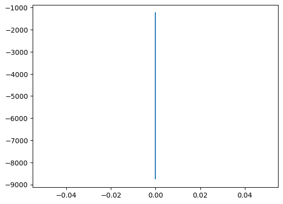
plt.plot(vx * (60 * 60 * 24 * 365.25), -y)
plt.show()
A is:
 [[1. 0. 0. 0. 0.]
 [0. 0. 0. 0. 0.]
 [0. 0. 0. 0. 0.]
 [0. 0. 0. 0. 0.]
 [0. 0. 0. 0. 1.]]
b is:
 [ 0.00000000e+00  0.00000000e+00  0.00000000e+00  0.00000000e+00
 -3.16880878e-10]
---------------------------------------------------------------------------
LinAlgError                               Traceback (most recent call last)
Cell In[2], line 48
     44 if ny < 15:
     45     print("A is:\n", A, "\nb is:\n", b.T)
     46
     47 # Solve it!
---> 48 vx = solve(A, b)
     49
     50 # Plot it!
     51 plt.plot(vx * (60 * 60 * 24 * 365.25), -y)

File ~/checkouts/readthedocs.org/user_builds/introgm/envs/develop/lib/python3.14/site-packages/scipy/linalg/_basic.py:300, in solve(a, b, lower, overwrite_a, overwrite_b, check_finite, assume_a, transposed)
    295 x, err_lst = _batched_linalg._solve(
    296     a1, b1, structure, lower, transposed, overwrite_a, overwrite_b
    297 )
    299 if err_lst:
--> 300     _format_emit_errors_warnings(err_lst)
    302 if b_is_1D:
    303     x = x[..., 0]

File ~/checkouts/readthedocs.org/user_builds/introgm/envs/develop/lib/python3.14/site-packages/scipy/linalg/_basic.py:84, in _format_emit_errors_warnings(err_lst)
     81         ill_cond.append(f"slice {i} has rcond = {dct['rcond']}")
     83 if singular:
---> 84     raise LinAlgError(
     85         f"A singular matrix detected: slice(s) {singular} are singular."
     86     )
     88 if lapack_err:
     89     raise ValueError(f"Internal LAPACK errors: {','.join(lapack_err)}.")

LinAlgError: A singular matrix detected: slice(s) [0] are singular.
Calculating strain rates#
The strain rate in 2D is defined as
In our case the only relevant component is the shear strain rate \(\dot\epsilon_{xy} = \frac{\partial v_x}{\partial y}\) . Why?
Exercise - Finite difference strain rates#
Discretize the shear strain rate expression
Complete the script below so that it will loop over all the grid points, calculate the shear strain, and store it in the array
eHow does the resulting plot look like? Note that the shear stress is defined as \(\sigma_{xy} = \eta\dot\epsilon_{xy}\). Where is the shear stress smallest?
e = np.zeros(ny-1)

# TODO: Write here a for-loop that loops over the grid points
# and calculate the shear strain rate on every step
(...)
(...)
(...)

plt.plot(e, -(y[1:] + y[:-1]) / 2.0)
plt.show()
Velocity boundary conditions#
Like in the case of the heat equation, the FD formulation for the velocity field can have different boundary conditions:
No-slip:
Velocity parallel to the surface is fixed at zero
\(v_x = 0\)
Free-slip:
Shear stress at the surface is zero
\(0 = \sigma_{xy} = \eta\dot\epsilon_{xy} = \eta\frac{\partial v_x}{\partial y} \Rightarrow \frac{\partial v_x}{\partial y} = 0\)
Other:
Velocity is fixed at non-zero value
For example, \(v_x = a \neq 0\), also incoming/outgoing flow (\(v_y \neq 0\)) is possible (in 2D models)
We used cases 1 and 3 previously.
Exercise - Exploring the channel flow boundary conditions#
Discretize the free-slip boundary condition \(\frac{\partial v_x}{\partial y} = 0\)
If you want to apply this at the upper surface (i.e. at \(x=x_0\)), how would your system of equations change? How would the coefficients in the matrix \(A\) change?
Modify your script for the channel flow model, and change the upper surface velocity boundary condition from \(v_x=0\) to a free-slip boundary condition
How does the resulting velocity plot change?
How does the plot for shear strain rate change?