Cluster computing#
Performance of geodynamic models#
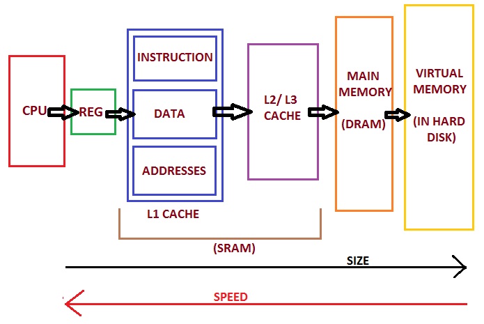
Memory hierarchy of modern PC (https://allthingsvlsi.wordpress.com)
Let’s consider a typical 2D thermomechanical geodynamic model:
Dimensions: 1000 km x 1000 km
Resolution: 1 km
Grid points: 1 000 000
Maximum time step (diffusion limit): 16 kyrs
Four unknowns: \(v_x\), \(v_y\), \(P\), \(T\)
Four equations per grid point
Discretized versions of the equations:
About 20 operations (
+,-,*, or/) per equationOperations per time step: 80 000 000
Modern PC processors can do about 10-100 GFLOPS (1 GFLOP = \(10^9\) floating-point operations per second)
The processor could do 1000 steps per second
For example, 50 Myrs / 16 kyrs per step = 3200 steps
Model run time: 3.2 secs
BUT: Memory access time (random): approx. 50 ns
Each operation needs to fetch at least one number from memory
Worst case: Random location
\(80\times10^6\times50\times10^{-9}~s=4.0~s\) per step
Total runtime (”wall clock time”): \(\approx 4~\mathrm{s/step}\times3200~\mathrm{steps}=3.5~\mathrm{hours}\)
Also, there is a lot of other “book keeping” during the model calculations
Exercise - How heavy is a 3D model?#
Make a similar runtime estimation for a 3D model with same resolution
Improving model performance#
A solution: Divide the job onto multiple processors.
Each will have fewer operations to do
Partitioning of the job:
Each processor will handle its own grid points, or
Each processor will handle its own part in solving the coefficient matrix
Each will have a smaller memory region to worry about (can store numbers closer to the processing unit)
Modern computer architecture#
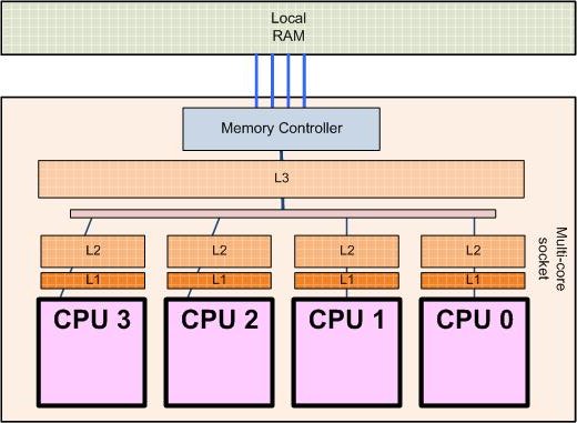
Processor architecture of a 4-core processor (http://sips.inesc-id.pt/~nfvr/msc_theses/msc10g/)
Modern PCs already use multiple cores (CPUs within one physical processor).
No speedup if the program/code used does not support multiple cores!
High-performance computing systems can have up to about 64 cores per CPU (typically), desktop computers normally have 2-8 (currently)
Some PC hardware allows two or more physical processors
More cores can be used by interconnecting multiple physical computers (nodes)
This requires a fast way to communicate between computers
Faster is better (>10 Gb/s)
Needs a protocol for CPUs/nodes to discuss with each other in order to distribute (partition) the work
One of the most common: MPI (Message Passing Interface)
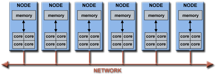
Architecture of a computing cluster
The geo-hpcc computer cluster#
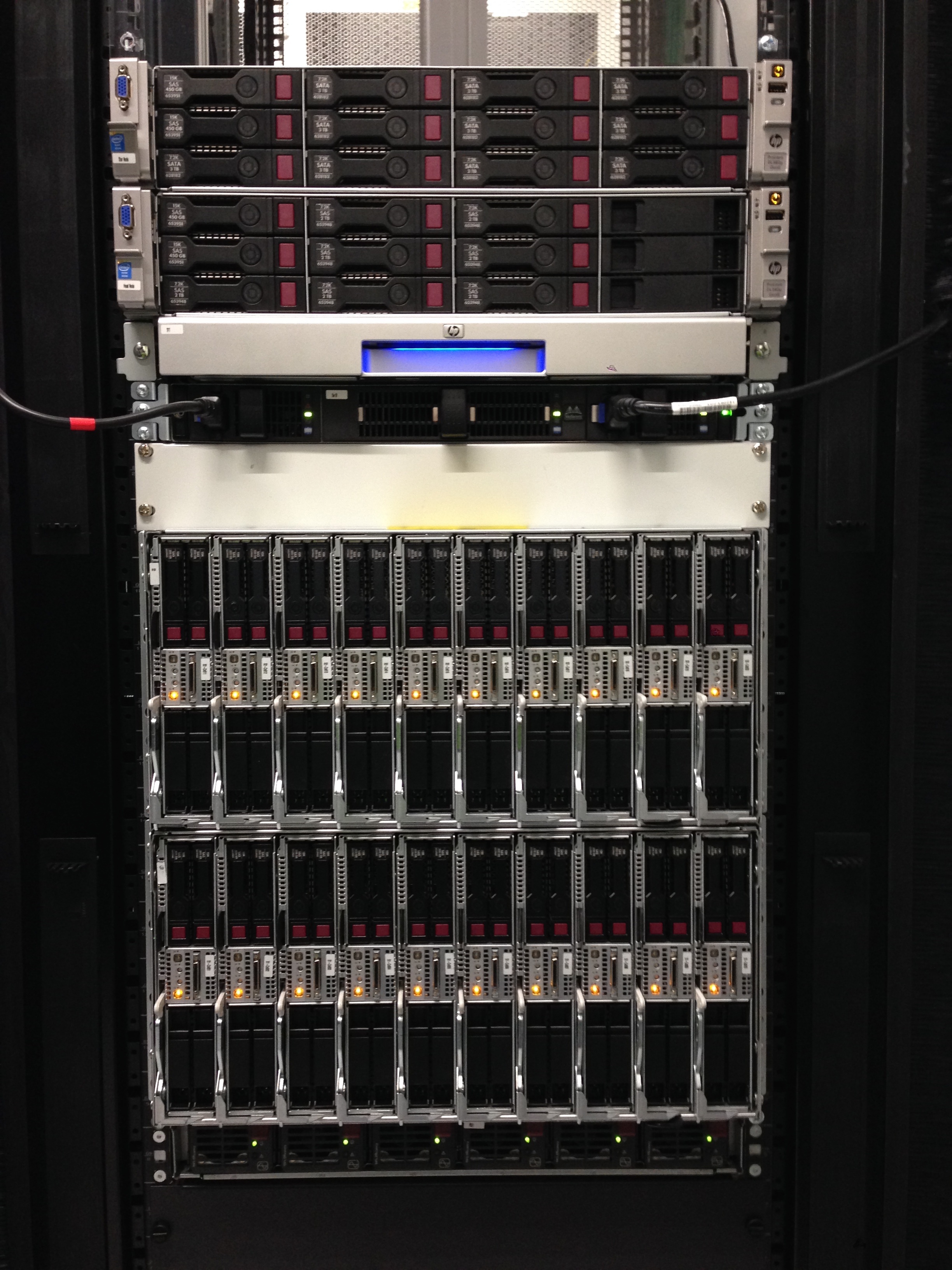
35 nodes, each with 2 processors, each with 8 cores = 560 cores
Performance of parallel programs#
We will test the effect of running a code in parallel, using the geo-hpcc cluster.
Login to the cluster using instructions on the course website
Type
mkdir mpi
cd mpi
cp /data/home/dwhipp/introgm/mpi/mpi.py .
spack load py-numpy py-mpi4py
srun -n 16 python mpi.py
To see and edit the Python code type
nano mpi.py
Exercise - Timing parallel performance#
Run the
mpi.pyscript with different number of cores (modify the number after-n, try values between 1-400 cores).Each time, record of the number of cores you use count and time it took for the calculation (with 4 decimal places for the time). We’ll compile our results and plot them as a group.
What kind of relationship would you expect to see?
What do you actually see?
Try commands
squeueandsinfoto see the job queue and the status of different nodes
Parallel performance results#
You can find the results of the parallel performance exercise in the exercise summary notebook.